SMM 2015

Welcome to my 2015 Marine Mammal Biennial page.  This page contains explanations of some of the work from the poster presented at the 21st Biennial Conference on the Biology of Marine Mammals. I've added some extra material here pertaining to the extraordinarily geeky components of my poster that wouldn't fit in the allotted space as well as some of the future directions the research will take.

You Might Be A Marine Mammal Scientist If....

Hi All [three of you]. I’ve been a horrible slacker lately and not updated anything. Part of this has to do with the fact that I’ve been working on a fairly cool project that’s almost ready for submission to a peer-reviewed journal, just waiting for my advisers to get some feedback to me… Once that's ready I look forward to sharing it here. In the meantime I’ve been thinking about what it means to be a marine mammal scientists, which I guess I should classify myself as since I’ve been unsuccessful in procuring gainful employment with any other species.

Personally, I’ve been interested in whales since I was a kid and have been privileged enough to have been born into a family that both pushed me in school and helped me, to the best of their abilities, pay for university. I’ve also been fortunate enough to have been supported by some great schools along the and by even better mentors (to whom I’m eternally grateful to). Anyway, for the last (eherm) 13 odd years I’ve been studying or working in the marine mammal field almost exclusively. Over that time I’ve noticed some interesting “particularities” and, dare I say it, bias among the marine mammal researchers. Some of these quirks are quite entertaining and others considerably less so. I’ve compiled them in a list of Jeff Foxworthy-esque statements. I hope you enjoy.

You might be a marine mammal biologist if:

If you’ve been reminded not to discuss whale necropsies at the dinner table.

I Need a Drink, the Cocktail Party Effect

This is a simple post explaining something most of us are quite familiar with already, social drinking. But don't worry, this blog-post is equally relevant to the abstainers among us. Incedently, Go Sober for October!

Actually, the cocktail party effect involves neither cocks nor tails (roosters people, get your mind out of the gutter). It is simply the natural ability to focus your perception on a single speaker when the room is full of conversations.

Sitting on a Cliff Waiting for some Dolphins

Notes From the Field

Hello all. I've just returned from a month in the Scottish highlands studying dolphins. Go ahead, you can be jealous and I'll forgive you. But it wasn't all fun and games, even before the tick bites and sunburns. I was there on a collaborative project with the University of Aberdeen Lighthouse Field Station (check them out and donate money) who are also studying dolphins using passive acoustic recorders.

The goal was to estimate the detection functions for  CPOD and SM acoustic detectors that comprise the majority of the data collection for my PhD.

Sitting on a cliff waiting for some dolphins...

Do You Hear What I Hear? Well, That Depends...

For the last few weeks something in the scientific literature has been irking me. As we've talked about before lots of skilled and dedicated researchers are now using passive acoustics to monitor animal populations. However, with all the acoustic recordings going on in the world and density estimations coming back, I see very few papers talk about how ambient noise levels will affect their monitoring ability and, ultimately, animal density estimations.  The core issues at play here are detection functions and maximum detection range (or radii). Both of these measures are greatly impacted by the ambient noise level.

What are detection functions and what is the maximum detection range?

But first we need to understand what these concepts are. Simply put, detection functions are a way to describe how likely a sound is to be heard the farther you are away from it. When the sound is very near you (or a recorder) we assume that there is a 100% chance of the sound being detected. But the greater the distance between the source and the receiver the lower the probability of detecting the sound. This proceeds until eventually the detection probability drops to zero. We will call the distance at which the detection function drops to 0 the maximum detection range.

For example, let's say you have a cricket (source) chirping in your ear (receiver).  Since the distance between the two is, essentially, 0 the probability of hearing a cricket calling while sitting in your ear is 100% . If the cricket hops 1 km away, you might expect that your probability of hearing it may drop to 50%. By 2 km the cricket chirps are so soft that it may be impossible to hear at all  (0% detection probability).

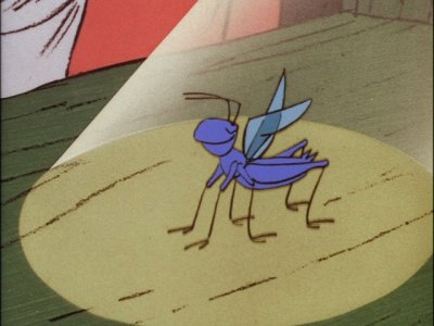
This is what the [overly] simple detection function for the cricket chirping might look like:

Very simple detection function because it makes the geometry easy (see below)

How many calls are missed?

From this figure we can see how the detacability of the cricket decreases with the distance away from the receiver. The interesting question then becomes, if we record X number of cricket chirps how many crickets were there in total? To answer this we need to know the ratio for the entire area monitored to the  (less than 2km) of the number of crickets we are likely to detect vs the number of crickets we are likely to miss. That is the ratio of the area under the red line to the total area monitored. In this example our detection function just happens to look exactly like a triangle (funny how that works) so now our probability of detecting the cricket within the maximum detection radius (2km) is ½*(b*h)/(b/h) or, 50%. Therefore, if we detect 150 chirps we might guess (based on the 50% detection probability) that we missed another 150. So the total number of cricket chirps that were actually there was 300.

A Little More Realistic-The Complex Acoustic Environment

Well isn’t that nice. Yes, too nice. That example was a complete fallacy and I bet you can guess some of the reasons why. First, the environment is complicated and sound scatters, bounces and is absorbed by things it runs into. If you have a microphone, or a point sensor, in the middle of a field but several crickets are chirping behind a very large stone, your probability from hearing crickets is much reduced. Similarly, if some crickets happen to crawl into the narrow end of a megaphone, their detectability goes up. Artists, scientists and mathematicians have known this for thousands of years and have exploited their natural surroundings to produce unique acoustic experiences.

Ambient Noise and the Area Monitored

The second major thing to consider is the noise level at the recording location. If a fighter jet were to fly over our recording station, the noise produced would have two effects. First, it would lower the probability of detecting the crickets by “masking” their sounds. Second, and what’s not often talked about, is that the noise will actually reduce the maximum detection range and therefore the total area monitored. This is a HUGE deal! Particularly for long-term studies looking at passive acoustics to estimate animal density. Let’s review from above. Animal density can be simplified to the following

Where N is the number of calls, C relates the number of calls to the number of animals (worthy of its own post) while Pdet and A are the detection probability and area monitored from above. So now, when the ambient noise level goes up the detection area (A) goes down. This will artificially inflate our density estimate. If you weren’t aware of that when you started analysing your data you might accidently report a higher density of animals than were actually there. No good.

Putting it All Together

Want to see how this might work in “real life”? Here I’ve used a propagation model and pseudo-simulated ambient noise levels to illustrate how noise might affect the total area monitored (Yes Doug, I know it’s not accurate yet but it serves to illustrate a point). If you watch the animation for a few seconds you can clearly that the area monitored is always changing. Similarly, you can see that sound doesn’t really pass into the red area. This is good, since the red area represents land and the rest is sea.

The consequences of this are pretty important, particularly when you are looking at things like habitat modeling. If, for instance a specific soniferous fish species (e.g. cod) preferred the deep channel just north of the sensor but you didn't consider whether that bit of habitat was included in your model, you might incorrectly surmise that cod prefer the shallow, near-shore waters. 

Don't Forget about Frequency

One last thing to talk about and that's the frequency of the sound. Lower frequency sounds generally travel further than higher frequency sounds because smaller wave lengths are more apt to be absorbed by the media, scattered and attenuated by the environment.

The above figure uses the same models and noise levels to demonstrate the area monitored at 40khz, rather than 5khz (as above). If you read the previous paragraph, this might seem like a contradiction. But, fortunately at higher frequencies there is less anthropocentric noise from ships, airguns, and construction. At 40 kHz the ambient noise is primarily dominated by wind and waves. So, in terms of monitoring higher frequencies are a bit of a double edged sward-the area monitored is smaller but it is likely less influenced by transient human activities.

So what does all this mean? It means that when doing density and abundance estimates or creating habitat models based on acoustic detections of animals it is important to acknowledge and, where possible, address the how the area monitored changes with the ambient noise.

R.O.C. On!

So, so much data.

One of the best, and worst, things about conservation acoustics is how easy and affordable it is to collect sound data. For the costs of paying one observer to sit in the field watching for animals, you could buy three or four acoustic recorders that can be used year after year. For any penny-pinching manager this is particularly enticing.

Unfortunately, while it is becoming ever easier to collect "gobs" of data it is also becoming more difficult to process it. For example, my PhD project will involve data collected  from 43 sensors every summer for four years. I estimate the total storage requirements to be over 40TB of acoustic data. To put that in perspective, the chemistry department in St Andrews was just gifted a server of the same size-for the entire department.

Anyway, as sometimes happens, thousands of dollars worth of recording equipment are purchased and deployed and one or two people are hired to process the data.

Admin1: Researchers are expensive but acoustics recorders are cheap.
Admin2: Then let's buy lots of recorders and hire one poor sop to process all the data.

Why Are Scientists So Obsessed With the Peer Review?

I recently got into an argument about the safety of the measles vaccine.

I’m quite fond of the person I was debating with so I tried to gently persuade them that the benefits of most vaccines outweigh the risks. I was also curious as to where they were getting their information from, particularly the so called studies that link autism to childhood vaccinations. I was happy that they were able to produce the reports but my heart sank when I realized the document she sent me was a work of pseudo-science.